 nn
nnConsider two independent finite samples {x1i}
i=1k and {x
2i}
i=1k of size k from
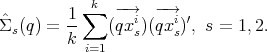
distributions F1 and F2 in n. Their sample covariances at point q  M, which
we refer to as an observation point, are
M, which
we refer to as an observation point, are
 n2×n2 be the mean and covariance of Z = (
 )(
)( )′, for X ~ F
s.
Thus, we assume that the mean and covarince of the tensor valued trandom
variable Z exist. As an application of the Central Limit Theorem we obtained the
asymptotic
)′, for X ~ F
s.
Thus, we assume that the mean and covarince of the tensor valued trandom
variable Z exist. As an application of the Central Limit Theorem we obtained the
asymptotic

![√-- -1 ′ T -1 ′
ξk(q;h) := k (h(ˆΣ1(q)ˆΣ 2 (q))- h (In )) ⇝ N (0,2[h(In)] (Ω ⊗Σ (q))[h (In)]),](comp4x.png) | (1) |
for similarity invariant h which gradient h′(.) n2 is continuous and does not
vanish at In. For example, ξk(q; tr) =  (tr(
(tr( 1(q)
1(q) 2-1(q)) - n) and
ξk(q; det) =
2-1(q)) - n) and
ξk(q; det) =  (det(
(det( 1(q)
1(q) 2-1(q)) - 1).
We apply bootstrapping method to utilize (1). For k′ < k, let ym,m = 1,...,M
be instances of statistic ξk(q; h) based on subsamples of size k′ of the initial
k-samples. The observation point q is chosen to be the sample mean of the
combined x1 and x2 samples. Then, according to (1), ξ =  ∕s.e.(y) goes to N(0, 1)
in distribution as k →∞.
∕s.e.(y) goes to N(0, 1)
in distribution as k →∞.
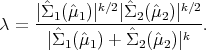
Another hypothesis of interest compares the usual covariances, defined at the
mean points H2 : Σ1(μ1) = Σ2(μ2). The corresponding likelihood ratio statistics
against the alternative Ha : Σ1(μ1) Σ2(μ2) is
 | (2) |
The exact distribution of λ is a product of independent Beta-distributions but can be approximated by chi-squared ones.
The following applet simulates distributions from different families and calculates ξ and λ statistics. The results are reported in term of p-values, Xi-pval for ξ and L-pval for λ. The user can choose the dimension n, sample size k and whether the two samples are equally distributed or not. Sub-sample size is fixed to k′ = k∕2 and M = k∕4. Possible choices for function h are the trace, determinant and h(A) = tr(log(A)). Shown are the two k-samples in red and blue and the observation point in green.