Tensor Response Envelope
Here we explain the basics of fitting an tensor envelope model with a tensor (multi-dimensional array) response Y on a multivariate predictor X.
Contents
Load the package
clear all;
cd D:\EnvelopeComputing\TensorEnvelope; % change directory to the package folder
setpaths;   % load all the functions in the package directory
rng(2015);  % set random seed
2D image response example
Regression of matrix-variate response image on scalar, binary predictor. The regression coefficients thus form a matrix image which can be visualized easily.
Load the image and resize the image to a 64-by-64 dimensional matrix with zeros and ones. Then use the image as the regression coefficient matrix B, and plot image in grayscale where 1's are in black and 0's are in white.
shape = imread('MPEG7/bat-7.gif');
shape = imresize(shape,[32,32]); % 32-by-32
b = zeros(2*size(shape));
b((size(b,1)/4):(size(b,1)/4)+size(shape,1)-1, ...
    (size(b,2)/4):(size(b,2)/4)+size(shape,2)-1) = shape; % 64-by-64
B = double(b);
imagesc(-B); colormap(gray);
title('Regression coefficient matrix')
axis equal;
axis tight;

Generate all parameters in the parsimonious tensor response regression model
r = [64 64];    % 64-by-64 matrix-variate response
m = length(r);  % m=2 (i.e. matrix) is the order of the tensor
p = 1;  % univariate predictor
rkB = rank(B);  % rank of B
u = [rkB rkB];  % envelope dimensions
n = 20; % sample size
B = tensor(B,[r p]);    % transform B into a tensor data-type
for i=1:2
    if i==1
        Gamma{i} = orth(double(B)); % Gamma1 spans the column space of B
    elseif i==2
        Gamma{i} = orth(double(B)');% Gamma2 spans the row space of B
    end
    Gamma0{i} = null(Gamma{i}');
    A = rand(u(i),u(i));
    Omega{i} = A*A';
    A = rand(r(i)-u(i),r(i)-u(i));
    Omega0{i} = A*A';
    Sig{i} = Gamma{i}*Omega{i}*Gamma{i}' + Gamma0{i}*Omega0{i}*Gamma0{i}';
    Sig{i} = Sig{i}./norm(Sig{i},'fro');
    Sigsqrtm{i} = sqrtm(Sig{i});
end
Generate the data from the model.
SNR = 0.1;  % signal-to-noise-ratio
Xn = [SNR*ones(1,n/2),zeros(1,n/2)]./norm(double(B),'fro');
Epsilon = tensor(normrnd(0,1,[r n]));
Epsilon = ttm(Epsilon,Sigsqrtm,1:m);
Yn = Epsilon + ttm(B,Xn',m+1);
Fit the voxel-based OLS estimator and the tensor envelope estimator.
[Btil1, Bhat1] = Tenv(Yn,Xn,u);

% Generate another data set with stronger SNR and fit the model.
SNR = 1;
Xn = [SNR*ones(1,n/2),zeros(1,n/2)]./norm(double(B),'fro');
Epsilon = tensor(normrnd(0,1,[r n]));
Epsilon = ttm(Epsilon,Sigsqrtm,1:m);
Yn = Epsilon + ttm(B,Xn',m+1);
[Btil2, Bhat2] = Tenv(Yn,Xn,u);
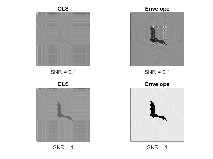
Plot the OLS and the envelope estimators under the two different SNRs.
subplot(2,2,1)
imagesc(-double(Btil1));
axis equal;
axis tight;
set(gca,'xtick',[],'ytick',[],'layer','bottom','box','on')
title('OLS')
xlabel(['SNR = ',num2str(0.1)]);
subplot(2,2,2)
imagesc(-double(Bhat1));
axis equal;
axis tight;
set(gca,'xtick',[],'ytick',[],'layer','bottom','box','on')
title('Envelope')
xlabel(['SNR = ',num2str(0.1)]);
colormap(gray);
subplot(2,2,3)
imagesc(-double(Btil2));
axis equal;
axis tight;
set(gca,'xtick',[],'ytick',[],'layer','bottom','box','on')
title('OLS')
xlabel(['SNR = ',num2str(1)]);
subplot(2,2,4)
imagesc(-double(Bhat2));
axis equal;
axis tight;
set(gca,'xtick',[],'ytick',[],'layer','bottom','box','on')
title('Envelope')
xlabel(['SNR = ',num2str(1)]);
colormap(gray);
P-value maps
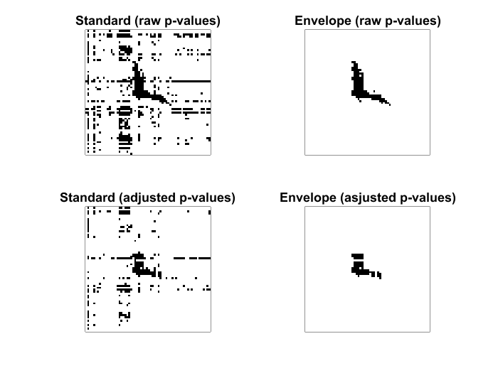
We implemented procedures for obtaining p-values of each elements in the tensor regression coefficient estimator. Two-sided t-testsare applied on both OLS and envelope estimators, where both use the asymptotic covariance of the OLS estimator. Both the raw p-values and the adjusted p-values are available, where the adjusted p-values are based on the Benjamini-Hochberg (1995) procedure for controlling of the false discovery rate in multiple testing. The B-H procedure might be problematic in our setting, since elements of the regression coefficent tensor are correlated.
SNR = 0.1;
n = 50; % sample size
Xn = [SNR*ones(1,n/2),zeros(1,n/2)]./norm(double(B),'fro');
Epsilon = tensor(normrnd(0,1,[r n]));
Epsilon = ttm(Epsilon,Sigsqrtm,1:m);
Yn = Epsilon + ttm(B,Xn',m+1);
Get the raw and adjusted p-values for each elements of the matrix-variate regression coefficent estimators (for both OLS and envelope estimators, respectively) and plot the p-value maps where p-value<0.05 is black and p-value>0.05 is white.
adjust = 0; % raw p-values
[Ptil, Phat] = Tenv_Pval(Yn,Xn,u,adjust);
subplot(2,2,1)
imagesc(Ptil>0.05);
axis equal;
axis tight;
set(gca,'xtick',[],'ytick',[],'layer','bottom','box','on')
title('Standard (raw p-values)')
subplot(2,2,2)
imagesc(Phat>0.05);
axis equal;
axis tight;
set(gca,'xtick',[],'ytick',[],'layer','bottom','box','on')
title('Envelope (raw p-values)')
colormap(gray);

adjust = 1; % adjusted p-values
[Ptil, Phat] = Tenv_Pval(Yn,Xn,u,adjust);
subplot(2,2,3)
imagesc(Ptil>0.05);
axis equal;
axis tight;
set(gca,'xtick',[],'ytick',[],'layer','bottom','box','on')
title('Standard (adjusted p-values)')
subplot(2,2,4)
imagesc(Phat>0.05);
axis equal;
axis tight;
set(gca,'xtick',[],'ytick',[],'layer','bottom','box','on')
title('Envelope (asjusted p-values)')
colormap(gray);
3D example
Here we demonstrate the model fitting of a higher-order tensor response regression, where the response is a three-way tensor and the predictor is a vector. The tensor regression coefficient is thus a 4-way tensor with dimension  .
.
r = [20 30 40]; % dimension of the tensor response variable
m = length(r);  % m=3 is the order of the tensor
u = [8 6 4];    % envelope dimensions for each modes
p = 5;          % multivariate predictor vector
n = 100;        % sample size
eta = tensor(rand([u p]));
for i = 1:m
    Gamma{i} = orth(rand(r(i),u(i)));
    Gamma0{i} = null(Gamma{i}');
    A = rand(u(i),u(i));
    Omega{i} = A*A';
    A = rand(r(i)-u(i),r(i)-u(i));
    Omega0{i} = A*A';
    Sig{i} = Gamma{i}*Omega{i}*Gamma{i}'+Gamma0{i}*Omega0{i}*Gamma0{i}';
    Sig{i} = 10*Sig{i}./norm(Sig{i},'fro')+ 0.01*eye(r(i));
    Sigsqrtm{i} = sqrtm(Sig{i});
end
B = ttm(eta,Gamma,1:m);
Xn = normrnd(0,1,[p n]);
Epsilon = tensor(normrnd(0,1,[r n]));
Epsilon = ttm(Epsilon,Sigsqrtm,1:m);
Yn = Epsilon + ttm(B,Xn',m+1);
Fit the OLS and envelope estimators and report their estimation errors in terms of the tensor norm of the different between the true and estimated tensor regression coefficients.
[Btil, Bhat] = Tenv(Yn,Xn,u);
disp(['OLS estimation error is: ', num2str(norm(B - Btil))]);
disp(['Envelope estimation error is: ', num2str(norm(B - Bhat))]);
OLS estimation error is: 17.1085
Envelope estimation error is: 0.19751
Geting the p-value maps just as in the 2D example
adjust = 0; % raw p-values; change it to "adjust=1" for adjusted p-values
[Ptil, Phat] = Tenv_Pval(Yn,Xn,u,adjust);
disp(sum(sum(sum(sum(Ptil<0.05))))/numel(Ptil));
disp(sum(sum(sum(sum(Phat<0.05))))/numel(Phat));
    0.4402

    0.3624
BIC selection
We use a heuristic BIC-type criterion combined with the 1D envelope algorithm (Cook and Zhang 2016; JCGS) to select envelope dimensions. Recall that in the above example we have and 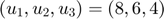 .
.
uhat = TensEnv_dim(Yn,Xn);
disp(u); % true envelope dimension
8 6 4
disp(uhat); % selected envelope dimension
8 6 4